Topics and Learning Outcomes
| Topics | After reading this Unit and completing the assigned readings in Physical Geology and the associated exercises and questions, you should be able to: |
|---|---|
| 4-1 Surface water and Groundwater |
|
| 4-2 Glaciation |
|
| 4-3 Mass Wasting |
|
Reading
Read Chapters 13 to 16 in Physical Geology.
4-1 Surface Water and Groundwater
Clean fresh water is our most precious resource. We cannot survive without it, and therefore, we should all know where our water comes from and what could put it at risk. In this first section of Unit 4, we will be looking at the water cycle, surface water, flooding, and groundwater.
Chapter 13 in the textbook examines streams and floods. We will be covering only part of that material in this section, including the hydrological cycle, flow of water on the surface, and the causes and effects of floods.
The hydrological cycle—illustrated in Figure 13.2 and described in Section 13.1—is familiar to most people. Water is stored in various reservoirs—the ocean, lakes and streams, soil and vegetation, glacial ice and groundwater—and is transferred from one to another with the help of energy from the sun (evaporation) and gravity (mostly stream and groundwater flow). Figure 13.3 provides two different ways of visualizing the amounts stored in these various reservoirs. The key point is that 97% of our water is salty water in the ocean, a further 2% is held in glacial ice, and fresh water that we can use makes up the remaining 1%. Over 90% of that is stored as groundwater.

You might find it instructive to do the experiment represented by Figure 13.3b in the textbook.
Pour 970 mL of water into a jug, and then add 34 g (7 teaspoons) of salt and stir. That’s how salty ocean water is. Taste it! A teaspoon won’t hurt you. Now add a single ice cube to represent all of the frozen water on Earth, and two more teaspoons of water to represent all of the water stored underground.
Now we need to add three more drops to represent the fresh water in all of the Earth’s lakes, streams, and wetlands plus all of the water in the atmosphere, including clouds. If you don’t have an eye-dropper, you could turn your tap down to the point where it’s just dripping, and capture three drops in a spoon.
Water moves between these reservoirs, and you can get a feel for the rate of transfer from one reservoir to another by completing Exercise 13.1.
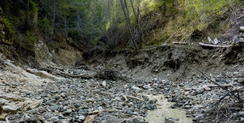
Groundwater is examined in Chapter 14, which begins with a discussion of porosity and permeability (Figure 4-3). As shown in Figure 14.2, most unconsolidated materials have porosities in the 30 to 60% range, whereas most solid rocks have porosities of less than 30%. Porosity is an important indicator of how much water can be held in rock or unconsolidated material, but the more significant factor that controls groundwater accessibility is the permeability of these materials, in other words, how easily water can flow through them.Section 13.2 examines the topic of streams and drainage basins, but you’ll only need to read the first few pages. A stream flows within a channel that is typically created by the stream itself through erosion of rock (Figure 4-1). A network of small streams that converge to make a large stream defines a drainage basin, which is an area of land within which all of the surface water eventually flows into the main stream. Drainage basins are illustrated in Figures 13.4 and 13.6.
Enlarge
© Steven Earle. Used with permission.
As discussed in Section 13.5, all streams show significant variations in discharge (volume of water passing a point per unit of time). In cold parts of Canada, the greatest flows are experienced in spring or early summer when melting is at its peak. This flow is illustrated in Figure 13.24 for the Stikine River in northwestern BC, which has a discharge of under 100 m3/s in the cold of winter, and peaks at over 2000 m3/s in May and June. In the southern coastal regions of BC, peak discharges are typically in mid-winter due to heavy winter rains (Figure 13.25).
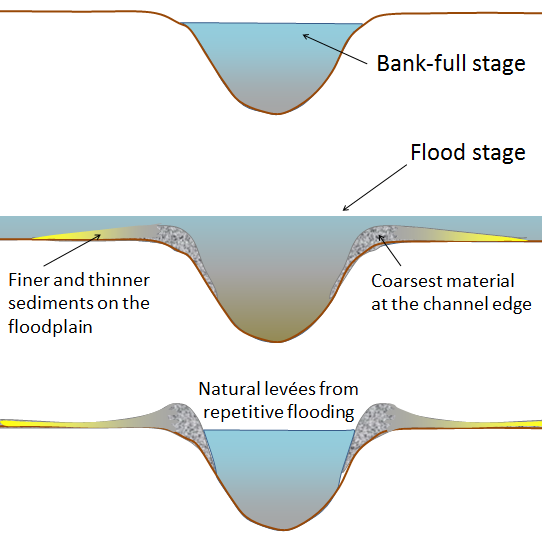
As a result of extreme rainfall events, or of rain storms that coincide with strong melting, discharge levels can be so great that streams fill their channels to the brim, and then spill over into the surrounding flood plain. This phenomenon is illustrated in Figure 4-2. The flow velocity reaches a maximum as a stream approaches its “bank full” stage, and then as soon as it pours over into the flood plain, the velocity drops significantly (because more area is available to accommodate the flow volume). When this happens, sediments are deposited on the banks and further out into the flood plain. The natural levees that form in these situations can help to limit future flooding. On many rivers, such as the lower part of the Fraser River, natural levees have been supplemented or replaced by man-made dykes.
Enlarge
Physical Geology by Steven Earle used under a CC-BY 4.0 international license.
Constructing dykes on rivers is controversial for many reasons. First it’s expensive, second dyking in one area can lead to flooding in other areas, and third flooding is what makes river-valley land fertile in the first place, so putting an end to floods is not in the best interests of farmers or the people that eat the food they produce.
In Section 13.5, read about the 2013 floods in southern Alberta, which, like many flood events in Canada, were caused by a combination of snow-melt and heavy rain.
Completing Exercise 13.5 will help you to understand the significance of this and other floods on the Bow River.
Answer the review questions 1, 2, 11, 12, and 13 at the end of Chapter 13, and check your answers in Appendix 2 in the textbook.
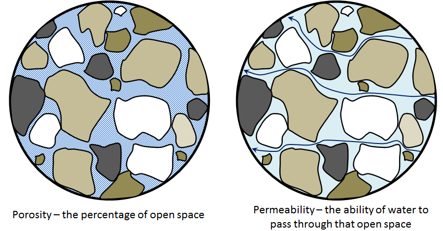
Groundwater is examined in Chapter 14, which begins with a discussion of porosity and permeability (Figure 4-3). As shown in Figure 14.2, most unconsolidated materials have porosities in the 30 to 60% range, whereas most solid rocks have porosities of less than 30%. Porosity is an important indicator of how much water can be held in rock or unconsolidated material, but the more significant factor that controls groundwater accessibility is the permeability of these materials, in other words, how easily water can flow through them.
Enlarge
© Steven Earle. Used with permission.
As shown on Figure 14.3, geological materials have a very wide range of permeability values from 0.000000000001 to 1 m/s (i.e., K = 10-12 to K = 100 m/s). Permeability is denoted by the letter “K.” Unconsolidated materials are generally more permeable than solid rocks, and the coarser they are, the more permeable. Unfractured igneous and metamorphic rock and mudstone have the lowest permeabilities, and well-fractured rocks tend to be much more permeable than unfractured rocks.
A strong correlation doesn’t necessarily exist between porosity and permeability. For example, while clay is one of the most porous of materials, it also is one of the least permeable. As described in the textbook, clay particles are very small and closely packed together. Its porosity is made up of many tiny spaces between the grains, and while those spaces can hold lots of water, almost all of it is tightly held by the mineral surfaces and cannot easily move within the clay deposit.
A body of rock or unconsolidated material that has good permeability is known as an aquifer, which is what people look for when they want to extract groundwater. The best way to find a good aquifer is to understand the geology of an area, and specifically the nature of the rocks and unconsolidated materials that might be underneath you. Of course this is not a guarantee that you’ll find what you’re seeking, since the permeability of a specific rock unit can vary from place to place. In some cases, permeability is related to fractures or bedding planes whose locations are very difficult to predict.
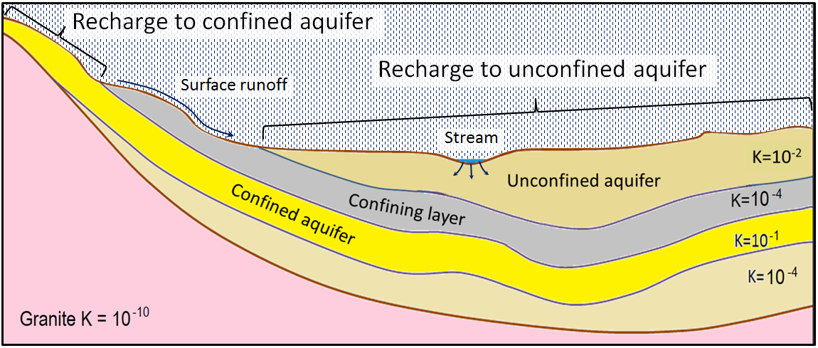
As illustrated in Figure 4-4 (which is similar to Figure 14.4 in the textbook), aquifers are described as unconfined if they are open to the surface, or confined if they are covered by a layer of impermeable material. In Figure 4-4, rain is depicted by vertical dashes, and a proportion of it will infiltrate into the ground and recharge the aquifer. Since an unconfined aquifer is exposed at the surface everywhere, it has more opportunity to be recharged by rain than a confined aquifer. An unconfined aquifer also can be recharged directly by a body of surface water (such as a stream) or by surface runoff.
Enlarge
Physical Geology by Steven Earle used under a CC-BY 4.0 international license.
The concept of a water table is introduced in Section 14.2, which describes it as the upper surface of a zone where all of the porosity is filled (i.e., saturated) with water. Be careful not to think of the water table as an object—you can’t pump water from a water table! However, you can pump water from a body of saturated rock, and the water table is just the upper surface of the part of that rock that is saturated. As shown in Figure 14.5, a water table isn’t typically horizontal. In this example, the water table is a few metres below the ground surface near to the top of the hill, but at surface, it is adjacent to a stream. The water table slopes towards the stream, and an 8 m difference exists in the elevation between the well and the stream. That difference in elevation, divided by the horizontal difference between the two points (100 m), is called the hydraulic gradient, which is denoted by the letter “i” (in this case, i = 8/100 = 0.08). The hydraulic gradient also can be described as the slope of the water table between those two points.
Section 14.2 also makes the point that if we know the hydraulic gradient and the permeability of an aquifer, we can estimate the rate of groundwater flow within an aquifer by using Darcy’s equation: V = K * i .
You can practice estimating groundwater flow rates and travel times by completing Exercise 14.1. Bear in mind that in this example and the one described in the textbook, the hydraulic gradients and permeabilities are on the high end of the spectrum found in nature. In other words, these flow rates—in the order of cm/day to m/day—are many times higher than would be typical in most natural settings.
Groundwater flow paths and rates are predictable, but not simple. Figure 14.8 shows that groundwater doesn’t flow in a straight line from an area where the hydraulic gradient is high to where it is low. Furthermore, in many situations, it can seem to flow “uphill.”
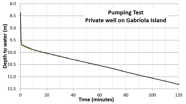
Extraction of groundwater is typically done using wells that are constructed in unconsolidated material or rock using a drilling machine like the one in Figure 14.10. Once the well has been completed, water can flow into it through the surrounding material, and a pump can be used to extract the water. As water is pumped out, it is typical for a cone of depression to form around the well (Figure 14.11), and if the pumping continues at a rate faster than the water can flow in, the well may go dry. In this case, when the pumping stops, the water level should recover.
An example of a water-level drawdown in a well during pumping is shown in Figure 4-5. When this low-capacity well was pumped at a relatively slow rate (3 litres per minute), the water level dropped from 8.4 m to 9.7 m in only 2 minutes, which produced a cone of depression of about 2.3 m that allowed the water to flow more quickly into the well. Nevertheless, the rate of inflow was not sufficient to keep up with the rate of pumping, and the water level continued to drop at a consistent rate for the next 2 hours.
Enlarge
© Steven Earle. Used with permission.
Wells are very useful for monitoring groundwater levels, and a large network of monitoring wells exists across British Columbia and elsewhere in Canada because it’s important for us to know the status of our groundwater resources. The well record shown in Figure 14.15 is typical for many wells in coastal British Columbia, with relatively high levels in the spring, peaking in April or May, dropping through the dry period of the summer and into the fall, and then starting to rise again in October or November. In colder regions, the peak comes later in the spring.
You can learn about the groundwater in your region by completing Exercise 14.3. If you don’t live in British Columbia, you may be able to find comparable data for your region.
Section 14.4 points out that groundwater has the distinct advantage of not being as easily contaminated as surface water—especially by bacterial contaminants—but the moderate disadvantage of having higher concentrations of many of the elements in surface water, in some cases, to dangerous levels and in others just to the extent that the water doesn’t taste as good as it should. Some examples are provided in the textbook.
It is critical for us to protect our groundwater resources because they are generally more reliable than surface water resources, and, as the climate continues to change, we may find that we cannot rely on our surface water supplies. One example of this shift is the rapid disappearance of glaciers everywhere in the world. In many locations, surface water supplies are significantly supplemented by the melting of glacial ice during the dry summer. Once those glaciers are gone, that component of the water supply will be gone too. Even where glacial melting is not part of the supply, snow melting typically is, especially in Western Canada. In recent years, snow packs have been at their lowest levels on record.
Please answer the review questions at the end of Chapter 14.
4-2 Glaciation
We are lucky to live during a time of glaciation because glaciers and their erosional effects are both spectacular and fascinating. They also hold a vast storehouse of information about the atmosphere and climate over the past several hundred thousand years. Even a few million years ago, glaciers were restricted to Antarctica and Greenland. Glacial ice did not exist anywhere on the planet 50 million years ago, nor for 200 million years prior to that. In addition, whereas many glaciations occurred in the distant past (Figure 16.2), the cumulative duration of glaciation on Earth represents considerably less than 10% of its history.
Section 16.1 discusses the history of glaciations, and Figure 16.3 summarizes the climate record of the past 65 Ma. As already noted, it was warm during almost all of the Mesozoic, and well into the Cenozoic, but the temperature started to change around 50 Ma as the collision between India and Asia created the massive Himalayan Range and Tibetan Plateau. The enhanced rate of erosion produced by this uplift increased the rate of chemical weathering of silicate minerals, and because that process consumes atmospheric carbon dioxide, the global temperature started to drop. A number of other tectonic processes, including the formation of other mountain ranges, contributed to a drop in global temperature of more than 12˚ C over the past 50 million years, and to progressively more glaciation, first in Antarctica, then Greenland, and finally over much of North America and Eurasia.
As shown on Figure 16.5, the Earth’s average temperature has fluctuated dramatically over the past few million years, swinging between glacial periods with mean global annual temperatures around 5 to 6˚ C, and interglacials—such as the present one—with mean annual temperatures around 12˚ C. Those relatively short-term fluctuations are related to small changes in the Earth’s tilt and the shape of its orbit around the Sun, known as Milankovitch Cycles.
Completing Exercise 16.1 will help you understand this cyclicity. In addition to answering the question asked, describe the nature of the temperature changes that preceded each of the past several glacial periods.
Section 16.2 in the textbook includes a discussion of the types of glaciers, and the mechanisms for glacier motion. Glaciers are of two types: alpine glaciers, which are present in mountainous regions, and continental glaciers, which cover entire continents. The only two real continental glaciers are those on Antarctica and Greenland. An ice cap glacier is similar to a continental glacier but covers less than 50,000 km2. They are present in Iceland, Svalbard, and the Canadian Arctic islands. An ice field is also a large area of ice, but one that is constrained by mountains. There are numerous ice fields in the Rockies and Coast Range of western Canada (Figure 4-6) and on the Arctic Islands.
Enlarge
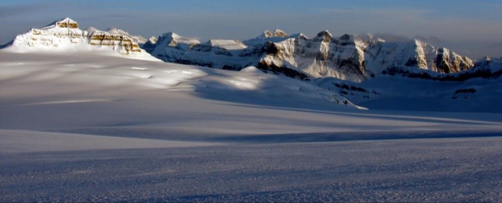
Hawthorne, R. (2011). Columbia Icefield view [Digital photo]. Wikimedia Commons. Retrieved from: https://en.wikipedia.org/wiki/Columbia_Icefield#/media/File:Columbia_icefield_view.jpg
As illustrated in Figure 16.13, glaciers move because the surface of the ice is sloped and also because the force exerted by the overlying ice causes the lower ice to flow as a plastic solid. The rate of deformation is greatest towards the base of the glacier, but because the overlying ice always moves along with the lower ice, the upper part of the glacier always moves faster than the lower part. An alpine glacier flows downhill, but that’s only because the surface of the ice is sloped in that direction (Figure 16.10). A continental glacier flows from the area of thickest ice towards the continental margin where the ice is thinner. In both cases, ice accumulates in the higher-elevation part of the glacier because in those areas, not all of the winter snow melts in the subsequent summer (in other words, the glacier is always covered in snow), and the ice flows towards the area where mass is being lost due to melting (a.k.a. ablation) or to the collapse of the leading edge. The boundary between the zone of accumulation and the zone of ablation is the equilibrium line, which can be easily observed on a glacier in late summer as the boundary between areas still covered in snow, and those with exposed (and melting) ice (Figure 16.12). Above the equilibrium line, snow is constantly being converted to ice through the process described in Figure 16.11.
Glacial ice may or may not slide across the rocky surface that it rests upon. If the base is warmer than the melting point of ice (because of heat flow from the rock beneath), a film of water will form between the ice and its base, and sliding is likely. If the base is frozen, sliding is unlikely, and all of the movement will be caused by internal deformation. Warm-based glaciers tend to move faster than frozen-based glaciers. The temperature at the base of a glacier is dependent on the average annual temperature in the region and the thickness of the ice.
At all stages in the life of a glacier (except when it is very small either because it is just starting to form or has nearly all melted away), the ice moves forward (down-slope in the case of an alpine glacier). Due to friction against the sides of the valley, an alpine glacier tends to move faster in the middle than at the sides (Figure 16.17). If the rate of production of new ice above the equilibrium line exceeds the rate of loss of ice below the equilibrium line, the glacier’s front end will advance. If those rates are the same, it will remain in the same place. If melting exceeds accumulation—as is the case with virtually all glaciers at present—the front end of the glacier will recede (Figure 4-7).
Enlarge
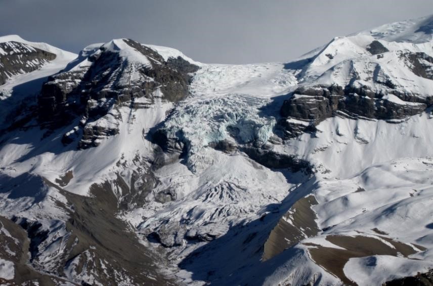
© Isaac Earle. Used with permission.
Completing Exercise 16.2 will help you to understand the processes of glacial motion and advance and retreat. Check your answer on the course textbook.
Section 16.3 summarizes the effects of glacial erosion, and as noted, continental glaciers produce substantially different erosional features than alpine glaciers. The key erosional landform of an alpine glacier is the U-shaped valley, with its steep sides and wide and relatively flat bottom, and the derivative features such as an arête that forms between two glaciers, a bowl-shaped cirque at the head of a U-shaped valley, a horn that forms between three or four cirques, and a hanging valley that is created where a smaller tributary joins a larger glacier that has eroded a deeper valley. Most of the important erosional features of alpine glaciation are illustrated from a variety of different perspectives in Figures 16.20, 16.21, 16.22, and 16.23 in the textbook, and also in Figure 4-8.
Take a close look at these figures and also complete Exercise 16.3 to help you ensure that you understand what alpine glacial erosion features look like.
Enlarge
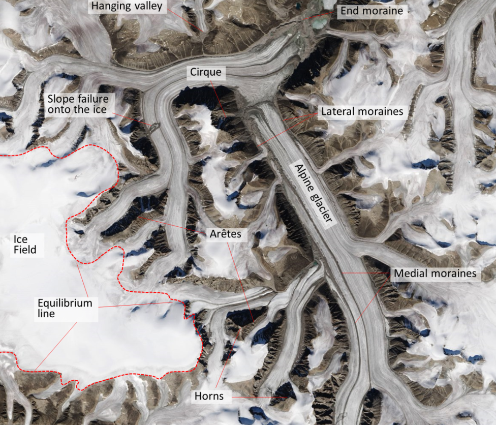
Adapted from Allen, J. (2015). Letter K: Sirmilik National Park [Digital image]. NASA Earth Observatory. Retrieved from: http://earthobservatory.nasa.gov/IOTD/view.php?id=87216&src=ve.
The striking erosional features of alpine glaciation are not created beneath continental glaciers. Instead, continental glaciers create vast areas that have been eroded to a nearly flat plain, although streamlined features, such as drumlins (Figure 16.19) and roches moutonée, and smaller features such as glacial grooves and striations (Figure 16.25) are common.
As summarized in section 16.4, glaciers transport sediments in wide variety of ways, including on top of the ice, within the ice, at the base of the ice; and perhaps most important of all, in running water on top, within, and beneath the ice (Figure 16.30). Some of the deposits associated with glaciers are unique to glacial environments, the most obvious being till, which is pushed along beneath the ice as lodgement till, or which rides along within or on top of the ice and is deposited as ablation till when the ice melts (Figure 16.31). The important and unique characteristics of till is that it is unsorted and does not typically show any layering. Glaciofluvial sediments are fluvial (stream deposited) sediments that accumulate in a glacial environment. In many cases, they look very similar to normal fluvial deposits, and the only evidence of their glacial origin is their age and location. In some cases, direct evidence of glaciation exists, such as the presence of layers of till, or dropstones from ice floating on glacial lakes and streams (Figure 16.35a). Glaciolacustrine deposits are typically fine sediments that accumulate in pro-glacial lakes, and typically have thin annual laminations related to summer and winter differences in meltwater production (Figure 16.35b).
Completing Exercise 16.4 will help you to understand where and how sediments are deposited in glacial regions. Some of the locations you are asked to identify may be underneath the ice.
Please answer the review questions at the end of Chapter 16.
4-3 Mass Wasting
Chapter 15 describes mass wasting as the gravity-related failure of material on slopes created by tectonic forces. Be sure to read the introductory section on what we can learn from past failures, such as the 1965 Hope Slide.
In Section 15.1, we look at the various factors that control mass wasting, including those that lead to slopes being unstable, and those that trigger specific mass-wasting events. One of the key issues is slope, because, as no one needs to be told, the steeper the slope is, the more likely that parts of it will fail. The physics behind this is illustrated in Figure 15.2. As steepness increases, the component of the gravitational force that is pushing material down the slope becomes greater. Where that force, known as sheer stress, exceeds the strength of the material, failure is possible.
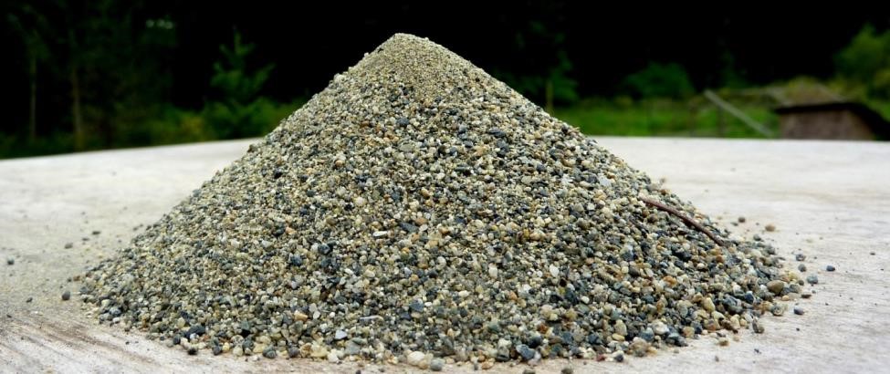
Therefore, the strength of materials on slopes is the other critical variable in slope failure, and that strength can vary for a number of reasons. The first factor is the overall strength of the material—whereas rocks like granite are extremely strong (and can form vertical slopes without failing), other rocks such as sandstone or mudstone are much less strong. Unconsolidated materials, such as glacial sediments, are even weaker because there is little to hold the particles together. Dry sand or gravel (or even cobbles or boulders) can only sustain a stable slope of around 30˚, as illustrated in Figure 4-9.
Enlarge
© Steven Earle. Used with permission.
Rock that is fractured or that includes bedding planes or metamorphic foliation is more prone to failure than solid rock, which is especially true if the fractures or planes of weakness are parallel to the slope (Figure 15.3). This potential for failure is also illustrated in Figure 15.1 and Figure 4-10.
Enlarge
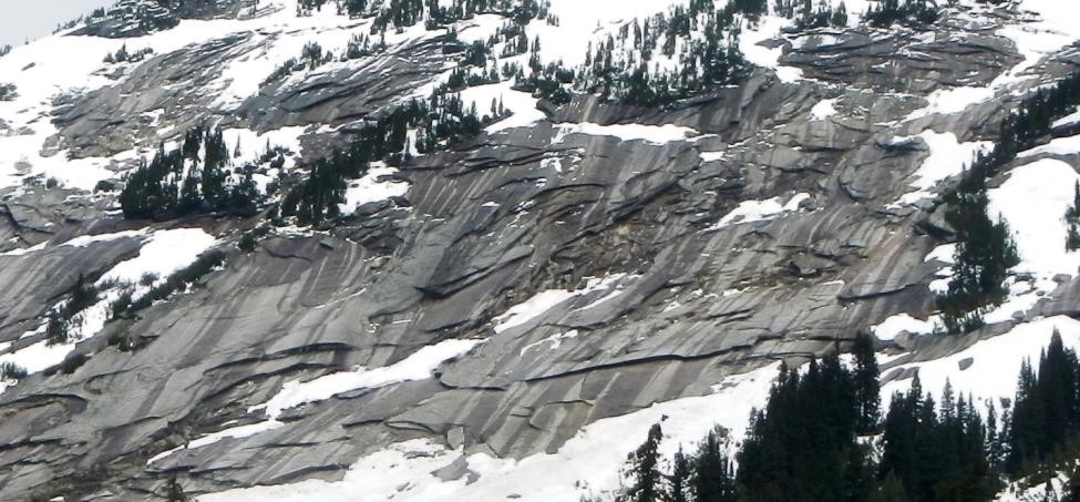
© Steven Earle. Used with permission.
Finally, water content plays an extremely important role in the strength of materials on slopes. With respect to unconsolidated sediments, a small amount of water—enough to coat the grains, for example—will have a cohesive effect that makes the material stronger than when it is dry. A large amount of water will push the grains apart, making the material weaker than when it is dry.
You can see this effect for yourself by completing Exercise 15.1.
Sediment with clay minerals are especially affected by water because these minerals can absorb water, which causes them to swell and weaken the material, thus facilitating failure.
Even the strength of rock is affected by the presence of water. As water under pressure fills fractures or bedding planes, it pushes the rock apart very slightly, which reduces friction along these planes and contributes to failure. That’s why you’ll see drainage pipes sticking out of solid rock along some highway road-cuts as shown in Figure 4-11. In such cases, holes are drilled for many metres into the rock to give water from fractures and bedding planes an opportunity to drain out.
Enlarge
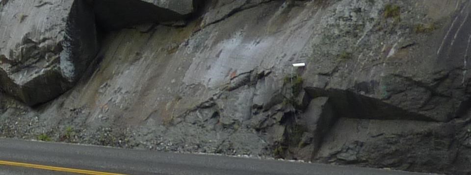
© Steven Earle. Used with permission.
Slopes can remain in a semi-stable state without failing for years or decades until some event triggers a sudden failure. As noted in the textbook, such triggers typically involve a weakening of the material, and the most common trigger is heavy rainfall that saturates and dramatically weakens unconsolidated material or even solid rock. In the example shown in Figure 15.6, heavy rainfall was a factor, but a disturbance to the drainage process related to roads, buildings, and landscaping in that built-up part of North Vancouver also contributed. Earthquakes also are common triggers of mass wasting because they shake and weaken geological materials.
The classification of mass wasting is summarized in Section 15.2. As noted, the key criterion for classification is the nature of the movement, which can be fall—if an object (such as a piece of rock) falls nearly vertically through the air; slide—if a body of material moves downslope as a single unit; and flow—if a mass of unconsolidated material or broken rock flows down a slope in a fluid manner. Of course it’s not always possible to know how something is moving, and it’s also quite common for more than one type of motion to occur during one event.
The classification of seven important types of mass wasting is summarized in Table 15.1. To familiarize yourself with these types, and the nature of their motion, complete the following exercise.
Seven types of mass wasting are listed below. Write each one in the most appropriate circle describing the type of motion.
| Slump | Fall | Slide | Flow |
| Creep |
 |
|
|
| Rock fall | |||
| Debris flow | |||
| Rock avalanche | |||
| Mud flow | |||
| Rock slide |
Please read carefully through the descriptions of the different types of slope failures in the rest of Section 15.2, and then complete Exercise 15.2, which should assist you in your understanding of the classification of slope failure.
The mitigation of risks associated with mass wasting is discussed in Section 15.3. It’s important to be clear from the outset that while we can delay some types of slope failure, for many years or even many decades, we cannot prevent it from happening. Erosion is inevitable and, in the long run, the efforts of mankind are insignificant. Even more important than trying to prevent mass wasting from occurring is to not make things worse through poorly planned construction, and to understand the mass wasting processes well enough to identify places that we should avoid.
As noted, road construction has a huge impact on slope stability, first because our road networks are so extensive, second because roads commonly have to cross difficult terrain, and third because roads require the creation of flat surfaces. Roads built along steep slopes inevitably make part of that slope steeper than it was, which increases the sheer stress and the risk of failure. Perhaps even more important, however, is that road construction impedes drainage on slopes, which typically weakens the material on the slope.
The construction of buildings and other structures also contributes to mass wasting, but not necessarily for the reason you might think.
Please complete Exercise 15.3, which deals with the effect of a building’s weight on slope stability as well as its effects on drainage.
In many cases, slope instability is recognized long before any significant threat of catastrophic failure, which gives us an opportunity to monitor a slope for any signs of change in its stability. The Downie Slide (Figure 15.9 and related text) is monitored this way. If any evidence occurs that its behaviour is changing, steps can be taken to reduce the risks downstream in places like Revelstoke. The lahar risk around Washington’s Mt. Rainier is monitored in different ways, but in this case, the warning time is measured in minutes instead of weeks or months.
In areas where we know that slope failures are inevitable, we can take steps to minimize risk. For example, the village of Lions Bay north of Vancouver is located on an alluvial fan, which is the only area flat enough to build houses in that part of a glacial U-shaped valley; however, it also is the worst possible place to build houses because the alluvial fan was built by hundreds of past debris flows. By the time the seriousness of the risk was recognized, dozens of expensive homes, a major highway, and a railway were sitting in harm’s way. Instead of moving everything, a decision was made to mitigate the risks by building containment structures, as illustrated in Figure 15.22.
Whenever possible, we should avoid the expensive measures of trying to prevent or delay mass wasting, or mitigate its effects as has been done in the Lions Bay area, and instead, keep infrastructure and people out of the way. An example of this avoidance strategy in the Garibaldi area in BC is provided at the end of Section 15.3.
Please answer the review questions at the end of Chapter 15.
This completes the notes for Unit 4.
Note if you are a registered student: If you haven’t already done so, now is the time to start working on Assignment 4. You should find most of what you need to complete the assignment within these course notes and Chapters 13 to 16 of your textbook, but you might also need to refer to other sources of information.